Written by Emil Hall on 23 August 2026.
This post is a contribution to the third Qualia Research Institute psychophysics retreat, which took place from May to June 2026 in Tepoztlán, Mexico.
Table of contents
QRI hereby publishes a computer simulation of the early stages of visual processing in the brain. The simulation is based on mathematical models from previous researchers, but extended with more features based on QRI’s phenomenological studies. We also relate it to QRI’s previous work on the “Oscilleditor” and the wider concept of coupling kernels in general.
Previous work
Probably the most well-known academic research about visual hallucinations is a series of papers by Paul C. Bressloff and Jack D. Cowan and sometimes other co-authors. Here are three of their papers:
Geometric Visual Hallucinations, Euclidean Symmetry, and the Functional Architecture of Striate Cortex - Paul C. Bressloff, Jack D. Cowan, Martin Golubitsky, Peter J. Thomas and Matthew C. Wiener. (2001)
What Geometric Visual Hallucinations Tell Us about the Visual Cortex - Paul C. Bressloff, Jack D. Cowan, Martin Golubitsky, Peter J. Thomas and Matthew C. Wiener. (2002)
Spontaneous pattern formation in Visual Cortex - Paul C. Bressloff and Jack D. Cowan. (2002)
We’re not going to go through the papers in detail here, but just to summarize, we could say there are two main parts to the model described in them. Firstly, the "retinotopic map", a coordinate transform between the visual cortex on one hand, and the retina (and subjectively experienced visual field) on the other hand. This math is relatively simple.
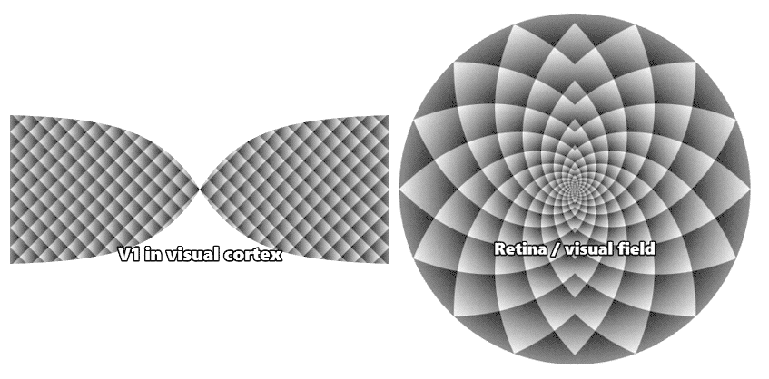
Drag to see the coordinate transformation
Secondly, an equation that describes how activity would evolve over time in the visual cortex. This is the mathematically challenging part. The authors used mathematical analysis to show that this equation has a bunch of steady-state solutions corresponding to visual patterns, here redrawn by us in higher quality:
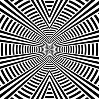
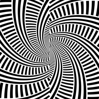
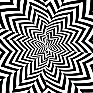
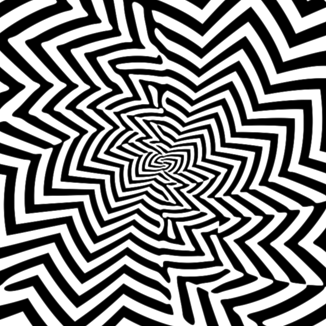
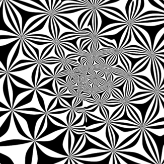
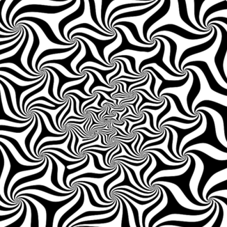
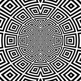
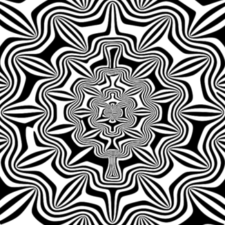
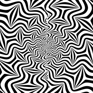
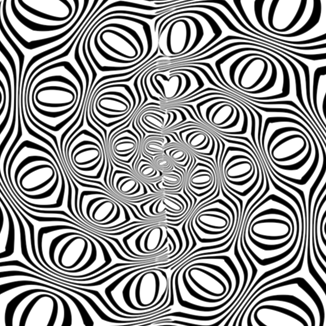
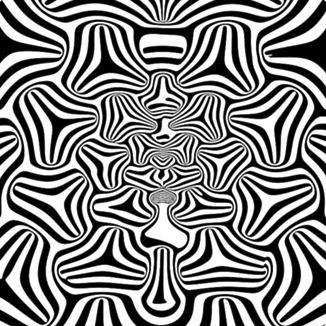
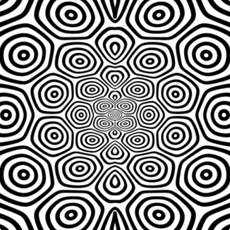
But something the authors didn’t do was to simulate the equation numerically. Maybe because when the papers were originally written, simulating the equation might have been unfeasible on anything less than a supercomputer, but now 25 years later any discrete GPU is powerful enough. A simulation has potential to be more interesting, because it can show more dynamic behavior that shifts over time, including unstable states. A simulation can also be easier to extend with more features.
Surprisingly, despite the advancements in computer performance, and despite the papers being so well known, the internet isn’t teeming with computer simulations of their model nowadays either. Maybe because the replication community is more artistic than mathematical? We found one simulation published on Github with 0 stars - not getting the attention it deserves.
Our simulation
So we implemented it. Here is a link to the full simulation which gives you full freedom to play around: Bressloff-Cowan V1 director field simulation
But it is quite hard to use, because it has a ton of parameters, and most parameter combinations don’t result in any patterns but just uncorrelated noise, 0 activity everywhere (blackout) or maximum activity everywhere (whiteout). We aim to publish a more polished version along with a detailed writeup in a few months.
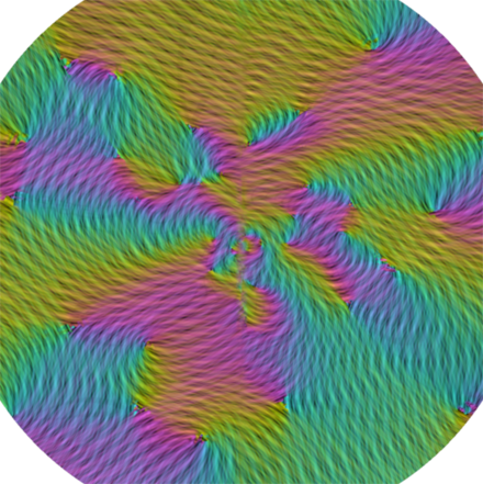
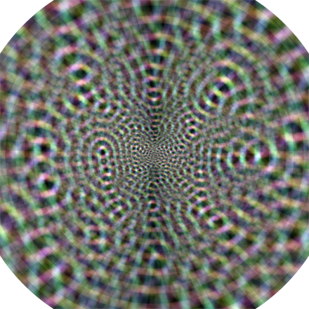
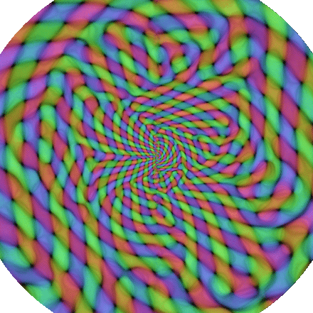
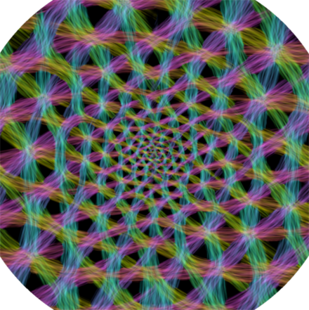
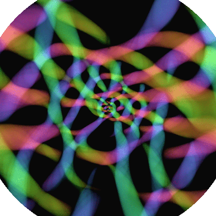
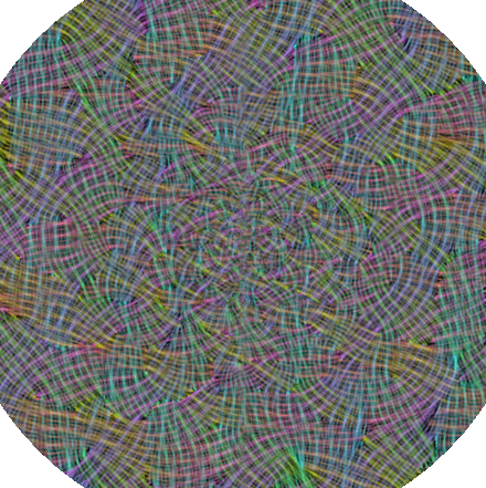
So here’s a gallery of some of the interesting patterns we have found so far:
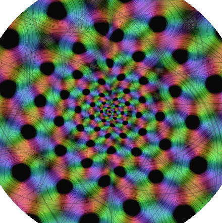
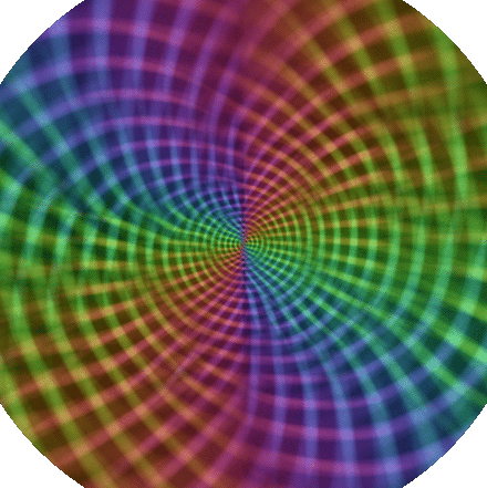
Coupling kernels and layers
Last year, QRI published the “Oscilleditor”. From the outside, it’s a tool to generate psychedelic visuals. From the inside, it’s a square grid of Kuramoto oscillators, where each oscillator is affected by its nearby neighbors in the grid. A coupling kernel decides exactly which neighbors affect it and how. That’s where the magic really happens - by varying the kernel, many different patterns can be generated. It’s more or less the same concept as a “convolution kernel” in artificial neural networks, or a “filter” in image processing (like a blur filter or sharpening filter), except that we keep applying the coupling kernel over and over again. QRI has written about coupling kernels before:
In the Oscilleditor, we actually have two separate grids or “layers” of oscillators, and each layer has its own user-defined coupling kernel. Then the two layers can interact, also with coupling, and we could have implemented this with one kernel for each interaction direction, bringing the total number of kernels up to 4, but to simplify we didn’t, we just hardcoded a 1-grid-cell-wide coupling between the layers.
Similarly, the most important parameters in the new simulation are the coupling kernels. Their effect is richer than in the Oscilleditor mainly because while the Oscilleditor has 2 layers, the new simulation has no less than 16. This means we could have 16*16=256 different kernels! That’s a vast parameter space, and obviously impossible to explore by manually designing 256 separate kernels. Fortunately, there’s some regular pattern to their shape that the research papers define based on anatomical studies on real brains. So our simulator’s GUI lets you edit the kernels on a higher level.
What are these 16 “layers”? They represent edges at different orientations. The brain has oriented edge detectors as a part of its curve completion mechanism. The number 16 is arbitrary, we just have to choose some number for computer simulation, just like we have to choose a grid width and height.
Is this an Artificial Neural Network? Depends on how strictly you want to define that term. Typical ANNs take in input that propagates through a number of layers one at a time, and some kind of result comes out the other end. But with a loose definition of terms, ours is closest to a recurrent neural network. Our layers don’t form a chain - there’s no input end and output end.
Limitations, current and future extensions
One thing we didn't see in the Bressloff-Cowan model was any parallel stripe patterns with empty space (inactive regions) in between, so we extended the model with a mexican hat kernel perpendicular to the oriented edge direction. Is that a thing that actually happens neurologically? Don’t know. Does it happen in subjective phenomena? Yes, definitely - at high dosages psychedelic visual patterns can consist of sharply defined edges, like isolines / contour lines, more or less evenly spaced.
Another limitation in their model is the discontinuity at the vertical line that goes through the center of the visual field. Since this “seam” is not experienced subjectively, there must be some neural circuitry (maybe later in the processing chain) which connects the left and right halves across the seam. The authors avoid the seam problem by generating their pictures on a simpler geometry, a plain log-polar space. We instead chose to use the more advanced geometry of the retinotopic map, which has the seam problem, and then we just added some arbitrary neural connections across the seam, and some color blending to further smooth out discontinuities.
We also added support for external input, i.e from the eyes. Because it’d be interesting to see how the model’s patterns get affected by external stimuli. For example, my own website hallucination-research.com has a plethora of experimental data on how hallucinations subjectively get affected by various inputs, so when the model matches such data, we can be confident it’s a good model. Currently, it doesn’t match very well. Why? See the last point below.
We also briefly tried adding support for co-circular kernels. There’s some debate in neuroscience about whether curve completion is accomplished by co-circular connection patterns on the neuron level, or if it’s a higher-level effect that relies on some feedback mechanism. We hoped that maybe co-circular kernels would help cause more curved patterns (matching our phenomenological observations), but they didn’t, and they complicated the simulation a lot, so we removed them again for simplicity.
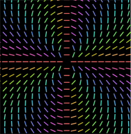
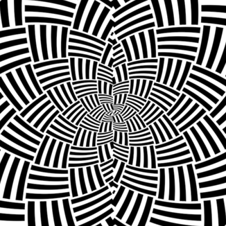
We also added support for “anti lateral kernels”, so where two lines would intersect at right angles, one of them tends to get suppressed. Is that a thing that actually happens neurologically? Don’t know. Does it happen in subjective phenomena? Yes, sometimes. Several retreat participants reported seeing “weave” patterns where “threads” would pass over or under each other - an effect that can be somewhat replicated with this kernel:
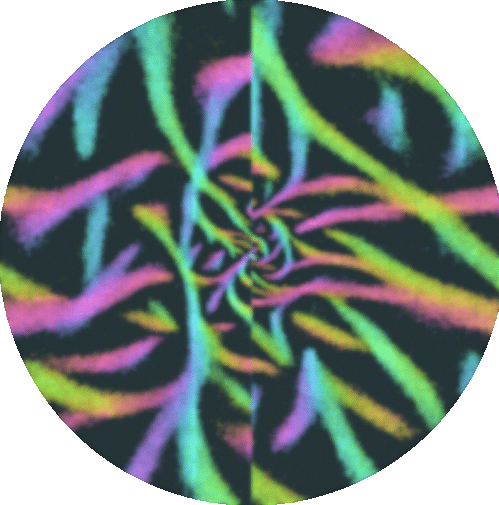
On the other hand, I personally saw a lot of travelling wavefronts that seemed to happily pass through each other at several angles, so it’s clearly not the case that line intersections get suppressed generally.
Which reminds me, another thing the model doesn’t support is travelling waves. It settles into stable patterns. We hope to soon add travelling waves by extending to the 2-population Wilson-Cowan model, where each cell in the field gets an “inhibitory” companion cell, and the normal “excitatory” cells increase the activity in the inhibitory cells, while the inhibitory cells suppress activity in the excitatory cells, thus forming a more dynamic system.
Finally, we can think of our 16 excitatory layers (and 16 future inhibitory layers) as forming just the “V1” part of the visual cortex, and more complex processing happens in V2, V3 and so on. Of course we should simulate that next level of processing too, although for each level there’s less and less neuroscience data on exactly what happens. We believe that comparing experimental simulation visuals to subjectively observed hallucinations will continue to be a powerful tool to figure out how the brain and the mind works.
Citation
For attribution, please cite this work as:
APA
Hall (2026, August 23). Simulating V1 following Bressloff, Cowan et al. https://heart.qri.org/retreats/2026-tepoz/emil-hall/bressloff-cowan-v1-simulation.html
BibTeX
@misc{hall2026bressloff,
  author = {Hall, Emil},
  title = {Simulating V1 following Bressloff, Cowan et al},
  url = {https://heart.qri.org/retreats/2026-tepoz/emil-hall/bressloff-cowan-v1-simulation.html},
  year = {2026}
}